A galactic-scale gravitational-wave detector
Millisecond pulsars are exceptionally stable clocks. A gravitational wave passing between Earth and a pulsar changes the apparent pulse arrival times by a tiny amount. Pulsar timing arrays combine years of timing residuals from many pulsars, searching for a common low-frequency process with the angular correlation predicted for an isotropic gravitational-wave background.
The characteristic Hellings–Downs correlation is the key population-level signature: pulsar pairs separated by different angles respond differently to the same stochastic spacetime perturbation. That makes a PTA more than a collection of independent time series. It is one correlated detector with irregular sampling, pulsar-specific noise, shared signals, and a likelihood whose covariance structure carries much of the physics.
Can PTAs detect gravitational-wave non-Gaussianity?
A background produced by a finite population of supermassive black-hole binaries need not be perfectly Gaussian. A small number of bright systems can create heavy tails, anisotropy, or other realization-dependent structure. A cosmological background may have different statistics again. This motivates a natural question: can model-agnostic distributional tests distinguish the underlying source populations directly from PTA measurements?
Our latest work follows that question from simulated populations to the effective PTA observables. The fastropop package generates ensembles of supermassive black-hole-binary populations and their nanohertz signals, making it possible to separate properties of the underlying sources from properties imposed by the PTA response. The largely negative answer is informative because it identifies which parts of the measurement erase the apparent differences—and therefore what a more targeted statistic would have to retain.
- Are PTA measurements sensitive to gravitational wave non-Gaussianities?Under review · arXiv:2605.05157v2
Chiara Cecchini, Jonas El Gammal, Gabriele Franciolini, and Mauro Pieroni.
Whitening is essential
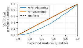
The samples entering a one-point distributional test are not independent. The gravitational-wave response induces correlations between pulsars, so applying an Anderson–Darling or Kolmogorov–Smirnov-type statistic directly to the correlated variables changes its null distribution. Apparent “non-Gaussianity” can then be produced by the covariance of an exactly Gaussian signal.
Whitening applies the inverse square root of the expected covariance, transforming the correlated Gaussian null into approximately independent unit-variance variables. Only after this step do nominal p-values recover their intended calibration. It is a basic statistical operation, but here it separates a property of the probability distribution from a property of the detector response.
Why most of the population structure disappears
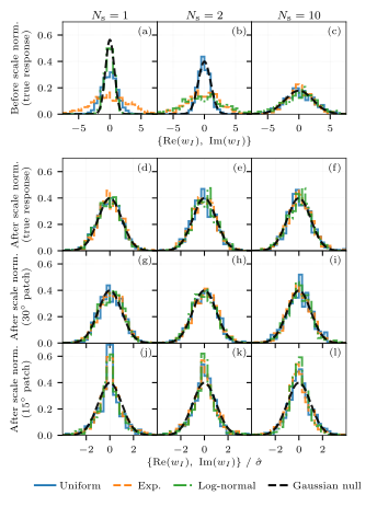
Two mechanisms account for most of the lost sensitivity. First, estimating the overall signal scale from the same realization removes variance information that would otherwise make two populations easy to distinguish. The test is then forced to use subtler shape differences rather than the amplitude of the fluctuations.
Second, each pulsar has a broad antenna pattern. Its timing residual receives contributions from a large fraction of the sky rather than resolving individual angular pixels. Summing many differently weighted source contributions pushes the effective response toward a Gaussian distribution, even when the underlying source map is visibly sparse or non-Gaussian.
This does not imply that all astrophysical backgrounds are exactly Gaussian or that source-population information is absent. It says that the model-agnostic one-point tests studied here have little power after covariance and scale are handled consistently. Statistics constructed around anisotropy, resolvable binaries, higher-order cross-correlations, or a specified population model are different—and potentially more sensitive—questions.